Computing mean average precision

Mean average precision or mAP is an object-wise metric to evaluate_generator the discriminative power of a detection model or a segmentation model.

Its computation involves two steps:

Matching the detections (or regressed object masks) to the best corresponding ground truth
Computing metrics according to the previously established matches

Matching detections and ground truths

Matching detections to ground truths can itself be divided into 3 steps:

Computing a pair-wise similarity index between each detections and each ground truths
Trimming impossible matches to rule out obvious mismatches
Doing the actual match based on the similarity index and the detection confidence score

The pair-wise similarity indexes are stored in a matrix called \(\mathcal{S}\) and the trimming is equivalent to working on the similarity matrix \(\hat{\mathcal{S}} = \mathcal{S} \circ \Delta\) where \(\Delta = (\delta_{i, j})\) is \(0\) on trimmed potential match and \(1\) elsewhere and \(\circ\) is the Hadamard product.

All these operations are performed by a MatchEngineBase object.

Computing the similarity matrix

The way we compute the similarity matrix depends on the geometric type of the detections and the ground truths:

If both detections and ground truths are either bounding boxes or polygons, the preferred method is Intersection over Union (IoU).
If either detections of ground truths are points, there are two possibilities:
- Using the euclidean distance between the points and the centroid of potential bounding boxes or polygons
- Assigning a fixed size box of polygon to each points and falling back to IoU

Intersection over union

Intersection over union or IoU—also called Jaccard index—is a measure of similarity between 2 sets.

As its name suggests it is defined as:

\[IoU = {{|A \cap B|}\over{|A \cup B|}} = {{|A \cap B|}\over{|A| + |B| - |A \cap B|}}\]

Where \(| \cdot |\) denotes the cardinal operator.

It may be extended as a geometrical similarity measure by considering \(A\) and \(B\) to be a set of point inside given shapes. Usually, we take \(A\) as the set of predicted points (as in a segmentation or a detection task) and \(B\) the set of ground truth points.

The IoU is thus defined as:

\[IoU = \frac{\mathcal{A}(A \cap B)}{\mathcal{A}(A) + \mathcal{A}(B) - \mathcal{A}(A \cap B)}\]

Where \(\mathcal{A}( \cdot )\) is the area operator.

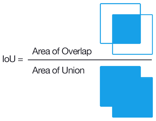IoUbbox Example of an IoU computation for bounding boxes (Credits: Adrian Rosebrock inIntersection over Union (IoU) for object detection)

The IoU is then used to determine how “close” the two shapes are. An IoU of 1 is equivalent to a perfect overlap, which is to say that the two shape are the same, whereas an IoU of 0 means no overlap and completely different shapes. Example: 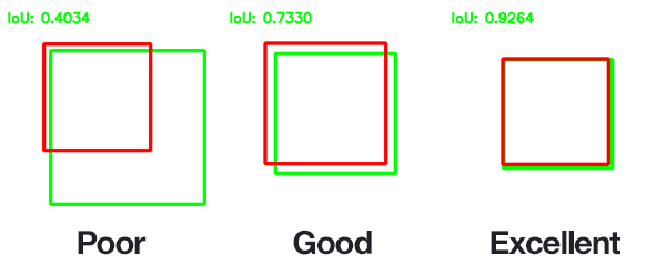IoUpoorgood Credits: Adrian Rosebrock inIntersection over Union (IoU) for object detection)

However, as one might see in the example before, the IoU decreases much quicker than overlap, which makes it very scrict metric when working with small objects.

Instance IoU

To alleviate this issue, the instance IoU or iIoU was introduced in the cityscape evaluation to correct the IoU by a coefficient of the area [1].

More precisely, the iIoU between a ground truth \(G_m\) and a detection \(D_n\) is defined as:

\[iIoU(D_n, G_m) = \frac{\overline{\mathcal{A}(G)}}{\mathcal{A}(G_m)} \cdot \frac{\mathcal{A}(D_n \cap G_m)}{\mathcal{A}(D_n) + \mathcal{A}(G_m) - \mathcal{A}(D_n \cap G_m)}\]

Where \(\overline{\mathcal{A}(G)}\) is the mean area of all ground truths of a given class in a given image.

iIoU has the advantage of lowering the impact of big ground truth instances while allowing small instances to be more easily matched.

[1] M. Cordts, M. Omran, S. Ramos, T. Rehfeld, M. Enzweiler, R. Benenson, U. Franke, S. Roth, and B. Schiele, “The Cityscapes Dataset for Semantic Urban Scene Understanding,” in Proc. of the IEEE Conference on Computer Vision and Pattern Recognition (CVPR), 2016.

Euclidean distance

The euclidean distance is the usual distance in euclidean geometry. It is defined as \(|| a - b ||_2 = \sqrt{\langle a - b, a - b \rangle}\) which in 2D euclidean geometry translates to \(\sqrt{(x_a - x_b)^2 + (y_a - y_b)^2}\).

As defined above, the euclidean distance is a dissimilarity index, the euclidean distant similarity index (EDS) is thus defined as:

\[\mathcal{D}(a, b) = 1 - \sqrt{(x_a - x_b)^2 + (y_a - y_b)^2}\]

Such that \(a=b \Leftrightarrow \mathcal{D}(a, b) = 1\) and \(\mathcal{D}(a, b) \in ]-\infty, 1]\).

Warning

This means that the EDS is not normalised, as opposed to the IoU and that the resulting similarity matrix is not sparse.

Trimming the similarity matrix

The similarity matrix has two type of trimming method types: threshold-based and membership-based.

The former is straightforward and consist in eliminating similarities below a certain threshold from possible matches.

It is used by the MatchEngineIoU, MatchEngineEuclideanDistance and MatchEngineConstantBox match engines.

The latter eliminate (det, gt) in which the detection is not inside the ground truth or vice-versa. The former is straightforward and consist in eliminating similarities below a certain threshold from possible matches.

It is used by the MatchEnginePointInBox match engine.

Matching

The matching contruct the match matrix \(\mathcal{M} = (m_{i, j})\) where \(m_{i, j}\) is \(1\) if the detection \(i\) is matched to the ground truth \(j\) and \(0\) otherwise.

There are two types of matching possible:

Unitary matching which imposes that a single detection can only be matched to a single ground truth.
Non-unitary matching which does not imposes any unity in the resulting matches: a ground truth could be matched to several detections and vice-versa.

Non-unitary matching

Straightforward match for all non-trimmed potential match, i.e. \(\mathcal{M} = \Delta\).

Unitary matching

Two match algorithms exist for unitary matches and yield different matches:

The Coco algorithm
The xView algorithm

Example case

Consider the following example where double boxes stand for ground truths with their id at their right and simple boxes for detection with their id and confidence at their right:

┌─────────┐ det1: 0.7
│         │
│    ╔════╪═════╗ gt1
│    ║    │     ║
└────╫────┘     ║
     ║          ║
     ║     ┌────╫────┐ det2: 0.5
     ║     │    ║    │
     ╚═════╪════╝    │
           │      ╔══╪═════╗ gt2
           └──────╫──┘     ║
                  ║        ║
                  ║        ║
                  ╚════════╝

The corresponding IoU similarity matrix is :

\[\begin{split}\mathcal{S} = \begin{bmatrix} 0.12 & 0 \\ 0.12 & 0.04 \end{bmatrix}\end{split}\]

Where each row corresponds to a detection a each column to a ground truth.

Matching algorithms

Coco match

Coco match runs trough all detections in decreasing confidence score. For each detection, we consider a valid match the higest similarity non previoulsy matched ground truth if its similarity is above a given threshold.

Consider the example above for an similarity threshold of 0.01:

We first look at det1 because it has the highest confidence, the biggest similarity in the first row of \(\mathcal{S}\) is 0.12 at the fisrt column. 0.12 is above the threshold and gt1 has never been matched to a detection before so we match det1 to gt1.

We then look at det2 because it has the second highest confidence, the biggest similarity in the second row of \(\mathcal{S}\) is also 0.12 at the fisrt column. However gt1 was previosly matched to a detection before so it is out of the picture, the second biggest similarity in the second row of \(\mathcal{S}\) is 0.03 at the second column. 0.03 is above the threshold and gt2 has never been matched to a detection before so we match det2 to gt2.

If the threshold is higher than 0.03, say 0.1, we would not be able to match det2 to gt2 meaning det2 and gt2 would not be matched to anything, couting respectively as a False Positive and a False Negative. Every matched detection count as a True Positive.

xView match

xView match runs trough all detections in decreasing confidence score. For each detection, we consider a valid match the higest similarity if its similarity is above a given threshold and the corresponding ground truth was never matched before.

Going back to our example:

We first look at det1 because it has the highest confidence, the biggest similarity in the first row of \(\mathcal{S}\) is 0.12 at the fisrt column. 0.12 is above the threshold and gt1 has never been matched to a detection before so we match det1 to gt1. Just the same as Coco so far.

We then look at det2 because it has the second highest confidence, the biggest similarity in the second row of \(\mathcal{S}\) is also 0.12 at the fisrt column. However gt1 was previosly matched to a detection before, det2 is thus left unmatched, meaning det2 and gt2 would not be matched to anything, couting respectively as a False Positive and a False Negative. Every matched detection count as a True Positive.

Example matching expected results summary

TP, FP, FN @ 0.01 similarity

Match strategy	True Positive	False Positive	False Negative
Coco	(`det1`, `gt1`), (`det2`, `gt2`)	0	0
xView	(`det1`, `gt1`)	`det2`	`gt2`

TP, FP, FN @ 0.1 similarity

Match strategy	True Positive	False Positive	False Negative
Coco	(`det1`, `gt1`)	`det2`	`gt2`
xView	(`det1`, `gt1`)	`det2`	`gt2`

Computation of mAP

Overview

The mean Average Precision is, as the name implies, the mean of Average Precision over labels.

Given a set of matched (detection, ground truth) couple (and possible unmatched elements, i.e. (detection, _) or (_, ground truth)), the Precision/Recall curve is computed using the PASCAL VOC [1] algorithm and the Average precision is defined as the integral of precision with respect to recall.

That is to say that given the \(P(R)\) function computed below:

\[AP_n = \int_{0}^{1} P_n(R) \; dR\]

And

\[mAP = \frac{1}{N} \sum_{n=1}^{N} AP_n,\]

where N is the number of labels (or classes).

Precision/Recall

Precision and recall for each label (or class) are defined as:

\[P_n = \frac{TP_n}{TP_n + FP_n} = \frac{TP_n}{D_n} \qquad R_n = \frac{TP_n}{TP_n + FN_n} = \frac{TP_n}{G_n} \qquad \qquad (1)\]

where \(TP_n\) represents the number of True Positive for the n-th label, \(FP_n\) represents the number of False Positive for the n-th label, \(FN_n\) represents the number of False Negative for the n-th label, \(D_n\) is the number of detection for the n-th label and \(G_n\) is the number of ground truth for the n-th label.

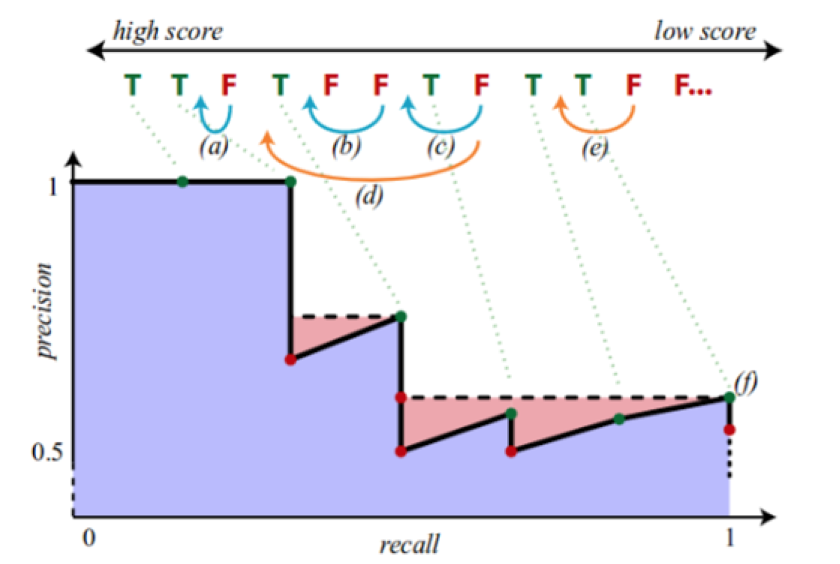
To compute the \(P(R)\) curve, the idea behind the PASCAL VOC algorithm [1] is to compute an approximate value of precision for increasingly high recall.

To do so, detections are sorted by decreasing confidence score. We start at the (1, 0) point and add detections one by one by following these rules:

If the detection is a True Positive, it has a positive effect on recall and precision according to \((1)\), we move by a G-th to the left and a D-th upward if precision is below 1.
If the detection is a False Positive, it has a negative effect on precision and no effect on recall according to \((1)\), so we move downward.

However this method compute an approximate precision for a given recall only and the following curve may be jagged. Before integration, we remove the jaggedness by interpolating a step function using at all recall value the maximum precision for all recall more or equal to the current recall.

The figure below illustrate the approximate precision computation as well as the anti-jaggedness interpolation:

ap_compute

[1] Henderson P., Ferrari V. (2017) End-to-End Training of Object Class Detectors for Mean Average Precision. In: Lai SH., Lepetit V., Nishino K., Sato Y. (eds) Computer Vision – ACCV 2016. ACCV 2016. Lecture Notes in Computer Science, vol 10115. Springer, Cham. https://link.springer.com/chapter/10.1007%2F978-3-319-54193-8_13